The Nobel Prize in Economics 2026 went to Robert E. Hall and Michael Woodford for rebuilding the models that governments and central banks use to steady an economy. Their central insight is that an economy is the sum of millions of decisions by households and firms, and those decisions depend on what people expect about the future.
Models built on this insight are now the main tool central banks use to decide interest rates. They replaced the post-war models, which failed in the 1970s when inflation and unemployment rose together.
Who Won the Nobel Prize in Economics 2026
The Royal Swedish Academy of Sciences awarded the prize on 12 October 2026 "for microeconomic foundations of macroeconomic stabilisation". Macroeconomic stabilisation means using interest rates, taxes and government spending to smooth out booms and slumps. Microeconomic foundations means building that analysis from how one household spends and how one firm sets prices, instead of from past statistical links between national totals.
Hall, born in 1943, is a professor at Stanford University. Woodford, born in 1955, is a professor at Columbia University. Their work connects directly. Hall's 1978 theory of household spending is the first equation in the model Woodford completed in 2003.
They share 12 million Swedish kronor and received the prize in Stockholm on 10 December 2026.
How the Great Depression and 1970s Stagflation Shaped Economic Policy
Stabilisation policy, the use of interest rates, taxes and government spending to smooth booms and slumps, has gone through three stages. It was born in the Great Depression, became standard practice after the Second World War and broke down in the 1970s.
What Keynes Argued and Why It Still Matters
The Great Depression was the economic collapse that began in August 1929 and lasted until 1941. Unemployment soared, and US prices fell by about 30% between late 1930 and early 1933. The British economist John Maynard Keynes argued that the slump came from a shortfall in total demand. When households and businesses stop spending, firms cut output and jobs. His remedy was for governments and central banks to cut rates and run budget deficits in a slump, and do the reverse when the economy overheats.
That core idea still underpins stabilisation policy. When the pandemic hit demand in 2020, the RBI cut the repo rate to 4.00% on 22 May 2020, and the US government mailed cash cheques to households. What changed after the 1970s is how policymakers decide how far and how fast to act.
How 1970s Stagflation Broke the Old Models
After the Second World War, Keynesian policy ran on models built from statistical patterns that looked stable. The best known was the Phillips curve, which says unemployment and inflation move in opposite directions. When jobs are plentiful, employers compete for staff, wages rise and prices follow. When many are jobless, wages and prices rise slowly. The British economist A.W. Phillips found this pattern in 1958 in UK wage data from 1861 to 1957. Many policymakers read the curve as a menu, believing permanently lower unemployment could be bought with modestly higher inflation.
That bargain failed. The West went through a decade of stagflation, meaning low growth, high unemployment and high inflation at the same time. Once households and businesses expected rising prices, they built them into wages and prices, so each step down in unemployment cost more inflation than the last.
The US Great Inflation 1965 to 1982 What happened. US inflation was just over 1% in 1964, passed 12% by 1974 with unemployment above 7%, and peaked near 15% in March 1980. Oil prices quadrupled during the Arab oil embargo that began in October 1973, and tripled again after the Iranian revolution of 1979. What changed. Paul Volcker became chair of the Federal Reserve in August 1979, with inflation above 11%, and tightened policy sharply from October 1979. The effect. Two recessions followed, the second running from July 1981 to November 1982, and unemployment peaked near 11%. Inflation fell below 5% by the end of 1982. As the Fed's commitment to low inflation gained credibility, unemployment fell and a long period of stable growth followed. |
Many people concluded from this decade that the stabilisation policy had done more harm than good. The lesson that stayed is that price stability comes first, and most central banks now have a numerical inflation target. India has had one since 5 August 2016. The target is 4% CPI inflation, with a tolerance band of 2% to 6%.
What Is the Lucas Critique
Robert Lucas, the 1995 economics laureate, showed why the old models failed. A pattern in past data holds only while policy stays the same, because people change their behaviour when policy changes. The Phillips curve proved it. When central banks pushed up inflation to cut unemployment, people came to expect more inflation, so inflation rose and unemployment did not fall. The fix was to build models on how households and firms decide, and Hall and Woodford built ones that still leave room for policy.
Robert Hall and the Random Walk Theory of Consumption
Hall settled a question that decides whether a stimulus works. He showed that households plan spending around what they expect to earn over their lifetimes, and change their plans only when genuinely new information arrives.
Why Household Spending Decides Whether a Stimulus Works
Household consumption is the largest part of demand in any economy, so every stabilisation decision depends on how households react to a change in income. Economists measure this with the marginal propensity to consume, the share of an extra rupee of income that people spend.
Before Hall, two answers stood far apart. The Keynesian view said people spend about two thirds of any extra income, so each rupee of government spending lifts output by about three rupees. Milton Friedman's permanent income hypothesis (1957) said people spend based on expected long run income, so they spend only about 2% of a one-time windfall each year. Under the first view a stimulus is powerful, and under the second it barely works. Friedman's view could not be tested, because no one could observe people's expectations.
How Hall Tested Forward Looking Spending in 1978
Hall found a way around the problem. If households already use everything they know about their future, today's spending already reflects it, and only news can change their plans. News cannot be predicted, so changes in spending should not be predictable either.
Hall tested this on quarterly US data. After accounting for current spending, past income had almost no power to predict future spending on non-durable goods. Economists call this the random walk of consumption, because each change in spending is as unpredictable as the news behind it.
What Are Hand to Mouth Households
Hall did not claim that everyone plans ahead. In 1982, with Frederic Mishkin, he studied the food spending of 2,309 US families between 1969 and 1975. About 80% of consumption followed the forward looking pattern, while 20% moved in step with current income. These are hand to mouth households, families with little savings or credit who spend whatever comes in.
Later evidence confirms the mix. Across studies of real government payments, households spent 21% of a one-time payment on average, or 11% after correcting for publication bias, the tendency of journals to favour striking results. A 1989 study of six advanced economies put the hand to mouth share near half of consumption. So a stimulus lifts spending more when it reaches households that spend what they receive, and models used by central banks and finance ministries now include both kinds of household.
💡What This Looks Like in Practice (Illustrative example) Say you receive a one-time bonus of ₹1,00,000.
|
Note: Illustrative example based on shares reported by the Royal Swedish Academy of Sciences, 1 Finance Research
Michael Woodford and the New Keynesian Model
Woodford built the New Keynesian model through papers in the 1990s and his 2003 book Interest and Prices. Its simplest version has three equations, each describing one forward looking decision.
- Households decide how much to spend. This is Hall's rule. A higher expected real interest rate, meaning the interest rate after inflation, makes people save more and spend less today.
- Firms decide their prices. Firms change prices only occasionally, which economists call sticky prices. So a firm resetting its price today builds in the costs and inflation it expects for the months ahead.
- The central bank sets the interest rate by a rule. When inflation rises, it raises its rate by more than the rise in inflation, which lifts the real rate and cools demand. This is known as the Taylor rule.
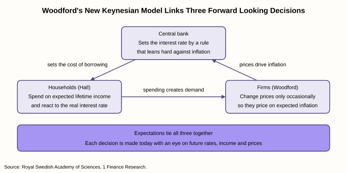
The central bank's rate shapes household spending, spending creates demand that firms respond to with prices, and inflation then feeds into the next rate decision.
How Central Banks Steer the Economy With Interest Rates
Older models treated monetary policy as control of the money supply. Woodford's model has no money in it. He drew on the Swedish economist Knut Wicksell, who in 1898 described a natural rate of interest, the rate that neither speeds up nor slows down the economy. A central bank steers the economy by setting its own rate above or below that natural rate. The vast majority of central banks now work this way. The RBI's tool is the repo rate, the rate at which it lends overnight to banks.
What Is the Output Gap
Woodford also gave policymakers the output gap, the difference between what the economy actually produces and what it would produce if prices adjusted freely. A positive gap means demand is running too hot and inflation will rise.
When energy prices jump, output falls, but the economy's potential output falls even further, so the gap can turn positive. The model then says to raise rates even as output falls. In the 1970s, the US Federal Reserve did the opposite and eased policy.
Why Central Bank Credibility Matters
Because households and firms look ahead, what people expect a central bank to do matters as much as what it does today. This is the basis of forward guidance, where a central bank tells the public how it expects to set rates in future. Woodford and others proposed forward guidance for times when rates sit at the zero lower bound, the point where rates are near zero and cannot be cut further.
Forward Guidance Examples From the US and India
The New Keynesian model had been in use for about a decade when the 2008 global financial crisis and the Great Recession that followed tested it.
| How Expectations Shaped Policy in the US and India | |||
|---|---|---|---|
| Episode | What happened | Policy response | Effect and lesson |
| US, August 2011 | The Fed's policy rate was already at 0% to 0.25% | The Fed said rates would likely stay exceptionally low "at least through mid-2013", replacing the earlier phrase "for an extended period" | A calendar date gave people a clearer view of the path ahead. Three members dissented in favour of the old wording |
| India, May to December 2013 | On 22 May 2013 the Fed signalled that it could slow its bond purchases | The RBI tightened liquidity in July and August 2013 and rebuilt buffers | The rupee hit a historic low at the end of August 2013. When the Fed acted on 18 December 2013, Indian markets withstood it better than other emerging markets |
| India, May 2022 to February 2023 | Crude oil traded above $100 a barrel during the conflict in Europe | The RBI raised the repo rate from 4.00% to 6.50% | The RBI tightened in a supply shock, the response the New Keynesian model recommends |
| India, October 2026 | CPI inflation rose to 4.8% in August 2026, and the RBI projected 6.0% for October to December 2026 | On 7 October 2026 the RBI raised the repo rate by 25 bps to 5.50% and shifted its stance from neutral to calibrated tightening | The RBI said rate cuts are off the table in the near term. This is forward guidance in practice |
The October 2026 statement uses Woodford's logic directly. The RBI said that monetary policy "primarily acts by curtailing second round effects", meaning it tries to stop a food and fuel price shock from spreading into wages and other prices.
What the New Keynesian Model Improved and Its Limitations
The new framework keeps Keynes's core insight, that demand matters and policy can help, while changing how the models are built.
| How the New Keynesian Model Improved on Older Models | ||
|---|---|---|
| Feature | Old Keynesian models | New Keynesian model |
| Foundation | Statistical links between national totals | Household and firm decisions, added up |
| Consumption | Fixed share of current income | Expected lifetime income, plus a measured hand to mouth share |
| Inflation | Fixed tradeoff with unemployment | Forward looking price setting and the output gap |
| Supply shocks | Stimulate to protect jobs | Tighten if the output gap turns positive |
The framework still has three known gaps.
| Limitations of the New Keynesian Model | ||
|---|---|---|
| Limitation | Why it matters | How research has responded |
| Households differ | Spending reacts to one-off income more than pure theory predicts, and differs across families | Models with many types of households and borrowing limits |
| The simplest model leaves things out | The three equation version has no investment, sticky wages or unemployment | Larger models estimated on data and used by central banks |
| Guidance needs credibility | An announced rate path changes behaviour only if people believe it | Numerical inflation targets that make intentions transparent |
India shows how guidance can change course. On 5 October 2018 the RBI held the repo rate at 6.50% and moved its stance from neutral to calibrated tightening. CPI inflation then fell to 2.2% in December 2018, its lowest in 18 months. On 7 February 2019 it cut the rate to 6.25%, returned to neutral and lowered its inflation projections. A stance signals intent based on current data, and the RBI changed it when the data changed.
Conclusion
Hall and Woodford revived stabilisation policy after the 1970s showed it could do real harm. Hall proved that most household spending looks ahead and measured the share that does not. Woodford built that insight, together with forward looking price setting, into the model central banks now use to set interest rates.
Central banks move the economy through expectations as much as through rates, and their words carry weight only while people believe them.